We are going to learn how to create and solve an exercice of the following type (and others more complicated than this without a doubt):
A carpenter has to construct rectangular tables whose sides do not exceed $$2$$ meters and that the sum of its biggest side and the double of the minor does not exceed $$4$$ meters. What is the maximum value of the perimeter of the above mentioned tables?
In this type of problem, the new part regarding what we have already seen in the previous levels, is that there appears a certain quantity that has to be maximized (it might also have to be minimized, but here this is not the case). In this example, it is the perimeter of the tables, which is subject to certain restrictions. The function to maximize (minimize) is called the objective function. The maximum value (or minimum) of the objective function is in the margins of the feasible area delimited by the restrictions of the problem. This value is called the ideal value.
Let's see how to express mathematically the problem of the example:
The first thing to be identified are the variables or unknowns. In this case those will be the long side of the table (that we will call $$x$$) and the short side of the table (that we will call $$y$$).
We identify the objective function. What we are asked to maximize / minimize? And: How does this quantity express itself according to the variables of the problem?
In our case we have been asked to maximize the perimeter (which we will call $$P$$) of the tables. The perimeter can be expressed as a function of the variables of the problem (long side and short side), since it is the sum of the double of every side. Mathematically: $$$P(x,y)=2x+2y$$$
Following the steps of the first level, we write the restrictions as inequations. These restrictions are:
-
The sides cannot be bigger than two meters (not even less than zero, since it would not make sense): $$$ x\geqslant 0 \qquad x\leqslant 2 \qquad y\geqslant 0 \qquad y\leqslant 2 $$$
- The sum of the biggest side and the double of the minor must not exceed $$4$$ meters: $$$ x+ 2y\leqslant 4$$$
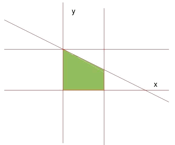
We identify the region of validity defined by the restrictions and calculate the apexes of the above mentioned region. The straight lines associated with the restrictions are:
- $$x=0$$ and $$x=2$$, which are straight lines parallel to the axis $$y$$, which cross $$x=0$$ and $$x=2$$ respectively. The inequality from which they come defines a stripe of feasible solutions between $$x=0$$ and $$x=2$$.
- $$y=0$$ and $$y=2$$, which are straight lines parallel to the axis $$x$$, which cross $$y=0$$ and $$y=2$$ respectively. The inequality from which they come defines a stripe of feasible solutions between $$y=0$$ and $$y=2$$.
- $$y=-\dfrac{1}{2}x+2$$, whose validity area is below the straight line (it is possible to see verifying that the poin $$(0,0)$$, which is below the straight line, fulfills the inequation $$x+2y\leqslant 4$$).

The apexes of the region of validity are calculated as in the previous level: looking at what points the straight lines defined by the restrictions cross one another and then select from these points those that satisfy all the inequations. Doing so, we see that the apexes of the region of validity take as coordinates:
-
$$(0,0)$$ where $$x=0$$ and $$y=0$$ cross.
-
$$(2,0)$$ where $$x=2$$ and $$y=0$$ cross.
-
$$(2,1)$$ where $$x=2$$ and $$y=-\dfrac{1}{2}x+2$$ cross.
- $$(0,2)$$ where $$x=0$$ and $$y=-\dfrac{1}{2}x+2$$ cross.
The last step is to calculate the value of the objective function in the apexes of the region of validity, to see which of the points maximizes the perimeter of the tables.
- $$P(0,0)=2\cdot 0+2\cdot 0=0$$
- $$P(2,0)=2\cdot 2+2\cdot 0=4$$
- $$P(2,1)=2\cdot 2+2\cdot 1=6$$
- $$P(0,2)=2\cdot 0+2\cdot 2=4$$
We see that the perimeter is maximized in the point $$(2,0)$$. The function perimeter takes there its ideal value, which is $$6$$ meters. The coordinates of the point are showing us that it will maximize the perimeter by making tables with long side ($$x$$) of $$2$$ meters and short side ($$y$$) of $$1$$ meter. We have already solved the first complete problem of linear programming.
Other examples:
The $$400$$ pupils of a school are going hiking. To do so, the trip hires a company that has $$8$$ buses of type A with $$40$$ seats and $$10$$ of the type B with $$50$$ seats, but there are only $$9$$ drivers for the day. Considering the different capacity and quality, the rent of every big bus (type B) costs $$80$$ € and each small bus (type A), $$60$$ €. How many buses of every class will it be necessary to rent so that the trip is as cost-saving as possible?
First, we identify the variables. In this case there will be the number of buses of type A (that we will call $$x$$) and the number of buses of the type B (that we will call $$y$$). The objective function is the price and it has to be minimized. The price according to the variables of the problem will be the sum of the price of a bus of type A (to $$60$$ €) multiplied by the number of buses of type A that are rented plus the same, but with the buses of type B (to $$80$$ €). Namely the price will be: $$$P(x,y)=60\cdot x+80\cdot y$$$
The restrictions of the problem in the form of inequations:
-
$$x\geqslant 0$$, $$y\geqslant 0$$ (we cannot rent a negative number of buses).
-
$$x\leqslant 8$$ ($$8$$ buses are type A).
-
$$y\leqslant 10$$ ($$10$$ buses are type B).
-
$$x+y\leqslant 9$$ (there are only $$9$$ drivers).
- $$40\cdot x +50\cdot y\geqslant 400$$ (we want the total number of places available to be at least equal to the number of students).
With the inequations, we do as we have done in level 2: look for the straight lines associated with the inequations, the areas of validity of every inequation and the common feasible area with all the restrictions.
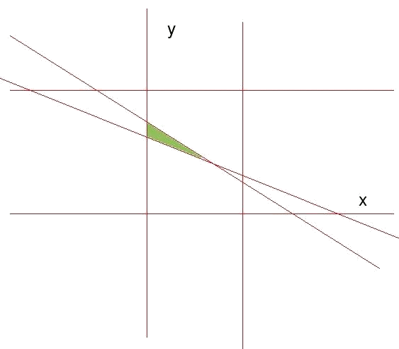
And the feasible area is:

The next step is to calculate the apexes of the region of validity. In this case they are: $$$ (0,8) \qquad (0,9) \qquad (5,4)$$$
The objective function (price) takes the following values in the apexes of the region of feasible solutions:
- $$P(0,8)=60\cdot 0+80\cdot 8=640$$ €
- $$P(0,9)=60\cdot 0+80\cdot 9=720$$ €
- $$P(5,4)=60\cdot 5+80\cdot 4=620$$ €
Since we want to minimize the price, the point that we want is $$(5,4)$$ and the price is $$620$$ €. Therefore, we will minimize the price if $$5$$ buses of the type A are rented ($$x$$) and $$4$$ buses of the type B ($$y$$) and everything will cost $$620$$ €.
To sum up, in any problem of linear programming we will have to follow the same steps:
- Choose the variables of the problem.
- Write the objective function according to the information of the problem.
- Write the restrictions as inequations.
- Determine the feasible region that the restrictions indicate.
- Calculate the coordinates of the apexes of the region of feasible solutions.
- Calculate the objective value of the function in each of the apexes to see in which of them the maximum or minimal value is available, as is asked in the problem.
