The continuous random variable $$X$$ follows a normal distribution $$N(\mu, \sigma)$$, being $$\mu$$ its mean and $$\sigma$$ its standard deviation, if it satisfies that:
- It can take any real value: $$(-\infty, +\infty)$$
- The probability density function (pdf) follows a gaussian curve:
$$$\displaystyle f(x)=\frac{1}{\sigma \sqrt{2\pi}}\cdot e^{-\frac{1}{2} \Big(\frac{x-\mu}{\sigma}\Big)^2}$$$
Find the PDF of a continuous variable with mean $$1,75$$ and standard deviation $$0,2$$ and represent it.
What could this distribution well represent?
$$$\displaystyle f(x)=\frac{1}{0,2 \sqrt{2\pi}}\cdot e^{-\frac{1}{2} \Big(\frac{x-1,75}{0,2}\Big)^2}$$$
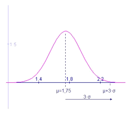
The given mean and standard deviation make this variable to be a good model of the heights of men in Barcelona.
To interpret the graph it is necessary to understand the probability that the variable takes a certain range of values in the area below the pdf curve in the given range or interval.
- The entire area of the pdf is $$1$$:$$$\displaystyle \int_{-\infty}^{+\infty} f(x) \ dx=1$$$
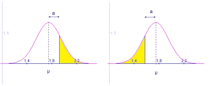
- The pdf is symmetrical with respect to $$\mu$$, that is to say, the area of each side of $$\mu$$ is $$0,5$$. Or, in the previous example, the number of persons over $$1,75$$m is the same as the number of people below the mean.$$$\displaystyle \int_{-\infty}^{\mu} f(x) \ dx=\int_{\mu}^{\infty} f(x) \ dx=\frac{1}{2}$$$
- Also the number of people taller than $$1,75 +a$$ is equal to the number of people under $$1,75-a$$
$$$\displaystyle \int _{-\infty}^{\mu-a} f(x) \ dx=\int_{\mu+a}^{\infty} f(x) \ dx$$$
The standard normal distribution
The standard normal distribution is the one that has mean $$\mu=0$$ and standard deviation $$\sigma=1$$:
$$$N(0,1)$$$
Its PDF is:
$$$\displaystyle f(x)=\frac{1}{\sqrt{2\pi}}\cdot e^{-\frac{x^2}{2}}$$$
In the following graph we see its representation:
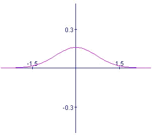
For the standard normal distribution it is possible to state:
$$$\displaystyle \int_{-\infty}^{0} f(x) \ dx= \int_{0}^{+\infty} f(x) \ dx = \frac{1}{2} \\ \int_{-\infty}^{-a} f(x) \ dx = \int_{a}^{+\infty} f(x) \ dx$$$
And it also satisfies all the properties of an even function, $$f(-x)=f(x)$$. Since the integral previously shown does not have an analytical solution, we use tables to calculate it.
Next, we can see the table corresponding to the values of the PDF, that is to say:
$$$p(Z \leq z)$$$
The first position of the table indicates the probability for the result of the experiment to give a value lower than zero (the average or mean) and we can see that this probability is $$0,5$$. The table shows that the probability of a result under a given value $$z$$ grows as $$z$$ grows.
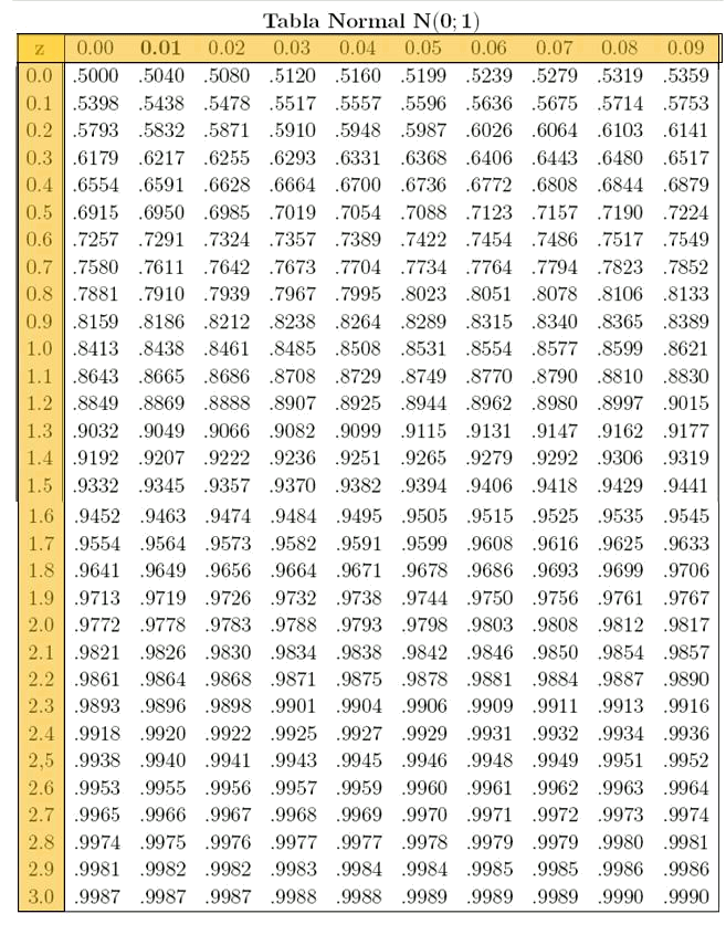
To read the table we must see that the column indicates the unit and the first decimal of $$z$$, while the row indicates the second decimal. Namely, in the first box of the first row the probability that we see is
$$$p(Z \leq 0,00)=0,5000$$$
while in the last box of the first row we see:
$$$p(Z\leq 0,09)=0,5359$$$
It can be seen that the table only gives the probabilities for positive values of $$Z$$. For values of $$Z <0$$ we will make use of geometry, as will be seen in the following examples.
It should be noted that after $$3$$ ($$3$$ times the standard deviation) the probability is very close to one ($$0,9987$$). Symmetrically, for values close to $$-3$$, the probability will be almost zero.
Find the probability of a random variable $$Z$$ modelled as $$N (0,1)$$ being lower than $$0,94$$.
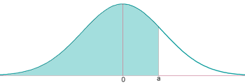
We have to look at the row of $$0,9$$ and the column of $$0,04$$:
$$$p(Z \leq 0,94)=0,8264$$$
Find the probability of a random variable $$Z$$ modelled as $N (0,1)$$ being greater than $$0,94$$.
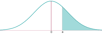
$$$P(Z \geq 0,94)= \mbox{Area}_{\mbox{total}}-P(Z \leq 0,94)\\ P(Z\geq 0,94)=1.0,8264=0,1736$$$
Find the probability of $$Z$$ being between $$0,94$$ and $$1,14$$
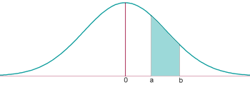
$$$p(0,94 \leq Z \leq 1,14)=p(Z \leq 1,14)-p(Z \leq 0,94) \\ p(0,94 \leq Z \leq 1,14)=0,8728-0,8264=0,0465$$$
Converting the standard normal distribution to any other normal distribution
What must we do to work with a normal distribution different from $$N (0,1)$$?
If $$Z$$ is a random variable $$N (0,1)$$ and $$X$$ is $$N (\mu,\sigma)$$, they are related by the following expression:
$$$\displaystyle Z=\frac{X-\mu}{\sigma} \\ X=\sigma\cdot Z + \mu$$$
We have a random variable with mean $$4$$ and standard deviation $$2$$.
What is its probability to be greater than $$6,21$$?
$$$p(X\geq 6,21)=p(\sigma \cdot Z+\mu \geq 6,21)\\ p(X\geq 6,21)= p(Z\geq \frac{6,21-4}{2})=p(Z\geq 1,105) \\ p(Z\geq 1,105) = 1- p(Z\leq 1,105)=1-0,8531=0,1469$$$
This way, only the tables for the standard normal $$N(0,1)$$ will be necessary.
Approximation of the binomial distribution from the normal distribution
For $$n$$ rather large, calculating a binomial $$B (n, p)$$ can turn out to be complicated. Then a normal distribution is used:$$$N(\mu=np, \sigma =\sqrt{npq}) \approx B(n,p)$$$
So, to deal with the binomial distribution corresponding to $$100$$ tosses of a coin, we can use:
$$$N(100 \cdot 0,5 , \sqrt{100\cdot 0,5 \cdot 0,5})=N(50, 5)$$$
Thus, we can avoid the calculation with high exponents that the binomial distribution would require and we will be able to use the tables for the normal $$N(0,1)$$.
